In this article we are going to use Scala mini-library for Deep Learning that we developed earlier in order to study basic linear regression task. We will learn model weights using perceptron model, which will be our single unit network layer that emits target value. This model will predict a target value yHat based on two trained parameters: weight and bias. Both are scalar numbers. Weights optimization is going to be based on implemented Gradient descent algorithm:

• Gradient Descent Optimization
• Training Loop

Model equation:

y = bias + weight * x

Data Preparation

Our goal is to show that perceptron model can learn the parameters, so that we can generate fake data using uniformly distributed random generator:

import scala.util.Random

val random = new Random()
val weight = random.nextFloat()
val bias = random.nextFloat()

def batch(batchSize: Int): (ArrayBuffer[Double], ArrayBuffer[Double]) =
  val inputs = ArrayBuffer.empty[Double]
  val outputs = ArrayBuffer.empty[Double]
  def noise = random.nextDouble / 5
  (0 until batchSize).foldLeft(inputs, outputs) { case ((x, y), _) =>        
      val rnd = random.nextDouble
      x += rnd + noise
      y += bias + weight * rnd + noise
      (x, y)
  }

val (xBatch, yBatch) = batch(10000)
val x = Tensor1D(xBatch.toArray)
val y = Tensor1D(yBatch.toArray)
val ((xTrain, xTest), (yTrain, yTest)) = (x, y).split(0.2f)

We have just prepared two datasets: 8000 data samples for train and 2000 samples for test cycles.

Model Training

First, we initialise sequential model for just one dense layer with single unit which is going to be a perceptron model.

val ann = Sequential[Double, SimpleGD](
  meanSquareError,
  learningRate = 0.00005f,    
  batchSize = 16,
  gradientClipping = clipByValue(5.0d)
).add(Dense())

In order to avoid exploding gradient values, we also set grading clipping value, so that whenever our gradient is not in -5;5 numeric range it will be clipped to left or right boundary accordingly.

Let's start training and see if real weight and bias which we used to generate fake data are learnt by the perceptron:

val model = ann.train(xTrain.T, yTrain.T, epochs = 200)

println(s"current weight: ${model.weights}")
println(s"true weight: $weight")
println(s"true bias: $bias")

Output:

epoch: 1/200, avg. loss: 1.205505132675171
epoch: 2/200, avg. loss: 1.0070222616195679
epoch: 3/200, avg. loss: 0.737899661064148
epoch: 4/200, avg. loss: 0.46094685792922974
epoch: 5/200, avg. loss: 0.2417953610420227
epoch: 6/200, avg. loss: 0.10201635956764221
epoch: 7/200, avg. loss: 0.037492286413908005
epoch: 8/200, avg. loss: 0.014684454537928104
epoch: 9/200, avg. loss: 0.00778685137629509
epoch: 10/200, avg. loss: 0.005894653964787722
....
epoch: 190/200, avg. loss: 0.005119443871080875
epoch: 191/200, avg. loss: 0.005119443871080875
epoch: 192/200, avg. loss: 0.005119443871080875
epoch: 193/200, avg. loss: 0.005119443405419588
epoch: 194/200, avg. loss: 0.005119443405419588
epoch: 195/200, avg. loss: 0.005119443405419588
epoch: 196/200, avg. loss: 0.005119443405419588
epoch: 197/200, avg. loss: 0.005119443405419588
epoch: 198/200, avg. loss: 0.005119443405419588
epoch: 199/200, avg. loss: 0.005119443405419588
epoch: 200/200, avg. loss: 0.005119443405419588

I have cut the middle part of the output, but it is not hard to see the progress.

Latest model weights:

weight = sizes: 1x1, Tensor2D[Double]:
[[0.690990393772042]]
,
bias = sizes: 1, Tensor1D[Double]:
[0.7804058255259821]

Original/true weights we used for data generation:

true weight: 0.7220096
true bias: 0.7346627

Numers are quite close to true numbers, but not exactly the same. I have set small/slow learningRate as 0.00005f by intention, so that our learning metrics will be smoother on the future plots. If we set learningRate to bigger value, it will be closer to true weights.

When I write weights I often mean bias and weight parameters in the same time.

Test dataset

We have 2000 data samples for model testing, let's what the error on predicting target values using unseen data:

val testPredicted = model.predict(xTest)  
val value = meanSquareError[Double].apply(yTest.T, testPredicted)
println(s"test meanSquareError = $value")

Loss value on test is quite close to training loss, so the learnt model is fine and we can continue:

test meanSquareError = 0.005048050195478982

Visualization

To visualize the loss function, I have decied to try Picta library. It can be used in Jupyter notebook via Almond Scala kernel, which is very cool.

Before we try to use Picta's 2D or 3D Canvas API, we need to prepare metrics data.

We could run the entire training code in Jupyter together with Picta around, but as of now Almond Scala kernel does not support Scala 3 which was used to write the Deep Learning code. So we will go with CSV files to bridge two worlds.

This is our plan:

1. Store metrics data from existing Scala 3 code to CSV files
2. Use CVS files in Jupyter with Scala 2.13

Data points vs. Model

Saving data points and gradient history, i.e. weight and bias during the training:

val dataPoints = xBatch.zip(yBatch).map((x, y) => List(x.toString, y.toString))
store("metrics/datapoints.csv", "x,y", dataPoints.toList)

val gradientData = model.history.weights.zip(model.history.losses)
    .map { (weights, l) => 
      weights.headOption.map(w => 
        List(w.w.as1D.data.head.toString, w.b.as1D.data.head.toString)
      ).toList.flatten :+ l.toString
    }
store("metrics/gradient.csv", "w,b,loss", gradientData)

store function is just creating a CSV file out of data in the Scala list:

def store(filename: String, header: String, data: List[List[String]]) =    
  Using.resource(new PrintWriter(new File(filename))) { w =>
    w.write(header)
    data.foreach { row =>      
      w.write(s"\n${row.mkString(",")}")        
    }
  }

Let's plot data points that we used to train the model as well the line that is based on learnt model parameters.

import org.carbonateresearch.picta.IO._
import org.carbonateresearch.picta._

val filepath = s"$metricsDir/datapoints.csv"
val data = readCSV(filepath)
val x = data("x").map(_.toDouble)
val y = data("y").map(_.toDouble)
val gradientData = readCSV(s"$metricsDir/gradient.csv")
val w = gradientData("w").head.toDouble
val b = gradientData("b").head.toDouble
def model(x: Double) = w * x + b
val m1 = Array(-0.1d, 1.3d)
val m2 = List(model(m1(0)), model(m1(1)))

val inputData = XY(x, y).asType(SCATTER).setName("Input Data").drawStyle(MARKERS)
val modelData = XY(m1.toList, m2).asType(SCATTER).setName("Model")
val chart = Chart().addSeries(inputData, modelData).setTitle("Data points vs. Trained model")

chart.plotInline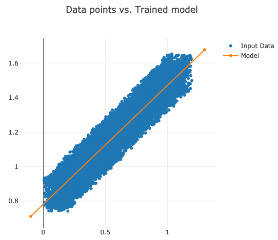

Our model crosses the data points almost in the middle as expected.

Loss metric per epoch

Creating a CSV file that contains loss value per training epoch.

val lossData = model.losses.zipWithIndex.map((l,i) => List(i.toString, l.toString))
store("metrics/lr.csv", "epoch,loss", lossData)

epoch,loss
0,1.205505132675171
1,1.0070222616195679
2,0.737899661064148
3,0.46094685792922974
4,0.2417953610420227
...

val metricsDir = getWorkingDirectory + "/../metrics"
val data = readCSV(s"$metricsDir/lr.csv")
val epochs = data("epoch").map(_.toInt)
val losses = data("loss").map(_.toDouble)

val series = XY(epochs, losses).asType(SCATTER).drawStyle(LINES)
val chart = Chart()
  .addSeries(series.setName("Learning loss"))
  .setTitle("Linear Regression Example: Loss vs. Epoch")
chart.plotInline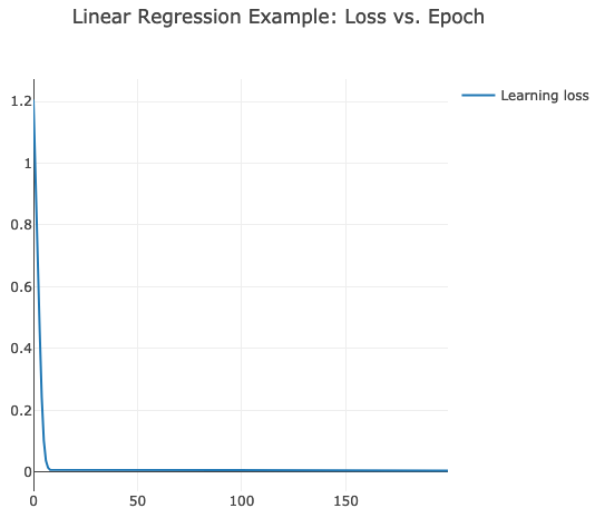

Loss Function Surface & Gradient History

Picta can also draw 3D plots, so that we can generate loss surface based on weight and bias parameters (x and y axis) and loss value as z axis.

val weights = for (i <- 0 until 100) yield i/100d
val biases = weights // we use the same range for bias
  
val losses = weights.par.map { w =>
  val wT = w.as2D
  biases.foldLeft(ArrayBuffer.empty[Double]) { (acc, b) =>
    val loss = ann.loss(x.T, y.T, List(Weight(wT, b.as1D)))  
    acc :+ loss
  }
}
 
val metricsData = weights.zip(biases).zip(losses)
  .map { case ((w, b), l) =>
    List(w.toString, b.toString, l.mkString("\"", ",", "\"")) 
  }
  
store("metrics/lr-surface.csv", "w,b,l", metricsData.toList)

w,b,l
0.0,0.0,"1.4736275893057016,... // here come 100 values for column `l` which stands for loss.
...

Last column is going to be used in 3D plot as Z axis. It is a list rather than a scalar value. This way we can draw a surface in Picta later.

val data = readCSV(s"$metricsDir/lr-surface.csv")
val w = data("w").map(_.toDouble).reverse
val b = data("b").map(_.toDouble).reverse
val loss = data("l").map(_.split(",").map(_.toDouble)).reverse
val surface = XYZ(x=w, y=b, z=loss.flatten, n=loss(0).length).asType(SURFACE).setName("Loss")

val gradientData = readCSV(s"$metricsDir/gradient.csv")
val gw = gradientData("w").map(_.toDouble).reverse
val gb = gradientData("b").map(_.toDouble).reverse
val gLoss = gradientData("loss").map(_.toDouble).reverse
val gradient = XYZ(x=gw, y=gb, z=gLoss).asType(SCATTER3D).setName("Gradient").drawLinesMarkers

val surfaceChart = Chart()
    .addSeries(gradient, surface)
    .setTitle("Loss Function Surface")
    .addAxes(Axis(X, title = "w"), Axis(Y, title = "b"), Axis(Z, title = "loss"))
surfaceChart.plotInline

Second plot gradient is for gradient history.

I have created several print-screens just to show you this beatiful surface from different angles:

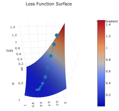
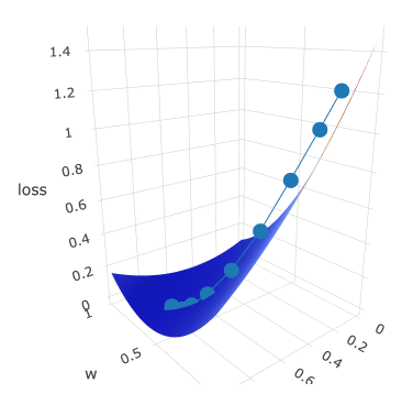
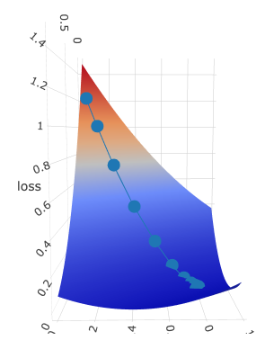
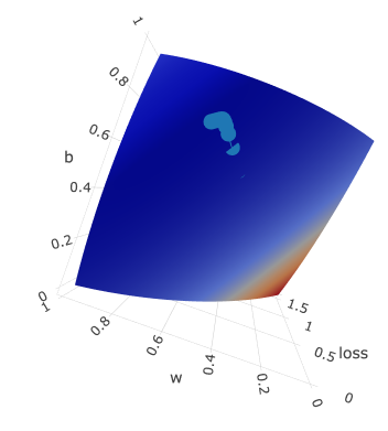
Dotted line is gradient descent trace: z axis is loss value which is moving to the local minimum with every epoch. It is moving according to its w and b, which are plotted on x and y axis accordingly.

Contour Chart

One more fancy chart from Picta is contour chart, which sometimes can be useful for analysis.

val contour = XYZ(x=w, y=b, z=loss.flatten, n=loss(0).length).asType(CONTOUR)
val contourChart = Chart().addSeries(contour).setTitle("Loss Contour")
             .addAxes(Axis(X, title = "w"), Axis(Y, title = "b"), Axis(Z, title = "loss"))

contourChart.plotInline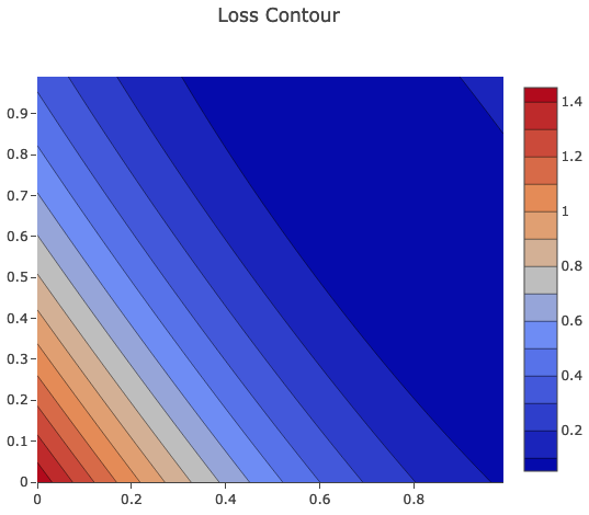

Just for you to prove that this was drawn in Jupyter actually :-)

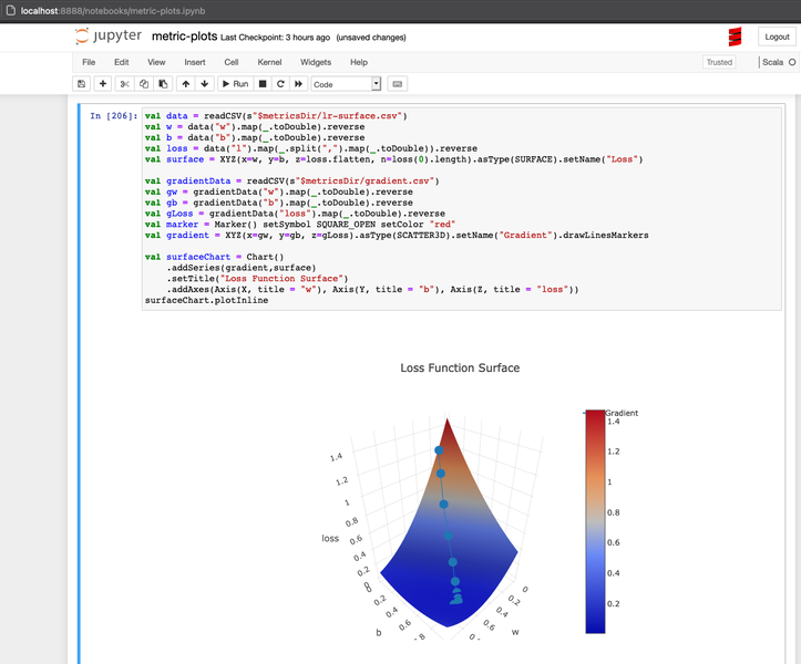
Again big thanks to Almond project that made Scala easily runnable in Jupyter.

Summary

We have seen that our perceptron model is able to learn weights very quick for simple 1 input variable. So it proves that gradient descent algorithm implemented earlier is working fine.

Also, we could visualise loss metrics using Picta and Almond Jupyter kernel for Scala quite easily. Such visualisation can help us to tune model training in real life use cases.