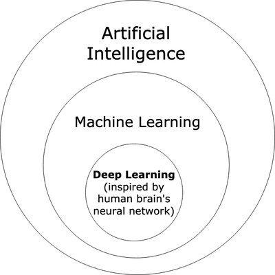
Deep Learning is a group of machine learning methods which are based on artificial neural networks. Some of the deep learning architectures are deep neural networks. Deep neural network is an artificial neural network (ANN further) with multiple layers between the input and output layers. There are different types of neural networks, but they always have neurons, synapses, weights, biases and functions.

Scala is a full-stack multi-paradigm programming language. Scala is famous for its innovations in JVM eco-system and ambitious language syntax features leaving all other JVM-based languages for years behind. Scala is also popular language thanks to Apache Spark, Kafka and Flink projects which are mainly implemented in it.

Scope

This tutorial is divided into 2 articles.

1. In this article we will go through the theory of ANN implementation. I will guide you through the basic calculus such as linear algebra and a little bit of differential calculus, which you need to know to implement neural network training and optimization algorithms.

2. In the second aritcle we are going to implement ANN from scratch in Scala. You can jump into second part directly, if you are familiar with the theory. But first look at the ANN Jargon table, if you decided to switch to second part.

ANN Jargon

I assume you are a bit familiar with Machine Learning or Deep Learning. Nevertheless, below table will be useful to match Deep Learning terminology with further Scala implementation. Some of the variable names in Scala code will be directly based on the Deep learning name definitions, so that it is important to know why some variable is named as z and another one as w.

Code Symbol / Type	Description	Encoded as
x	input data for each neuron	2-dimensional tensor, i.e. matrix
y , actual	target data we know in advance from the training dataset	1-d tensor, i.e. vector
yHat , predicted	output of the neural network during the training or single prediction	1-d tensor
w	layer weight, a.k.a model parameters	2-d tensor
b	layer bias, part of the layer parameters	1-d tensor
z	layer activation, calculated as x * w + b	2-d tensor
f	activation function to activate neuron. Specific implementation: sigmoid, relu	Scala function
a	layer activity, calculated as f(z)	2-d tensor
error	it is result of yHat - y	1-d tensor
lossFunc	loss function to calculate error rate on training/validation (example: mean squared error)	Scala function
epochs	number of iterations to train ANN	integer > 0
accuracy	% of correct predictions on train or test data sets	double number, between 0 and 1
learningRate	numeric parameter used in weights update	double number, usually between 0.01 and 0.1

Tensor

Deep Learning is all about tensor calculus. Tensor in computer science is a generic abstraction for N-dimensional array. In our ANN implementation, we are going to use scalar numbers which are encoded as 0-dimension tensor, vector - encoded as 1-d tensor and finally matrix - encoded as 2-d tensor. Vector and matrix are the most used building blocks for Deep Learning calculus. All tensor shapes we will use are going to be rectangular - every element is the same size along each axis.

Dataset

We will take _Churn Modelling dataset which predicts whether a customer is going to leave the bank or not. This dataset is traveling across many tutorials at the Internet, so that you can find a couple different code implementations among dozens of articles using the same data, so do I.

RowNumber,CustomerId,Surname,CreditScore,Geography,Gender,Age,Tenure,Balance,NumOfProducts,HasCrCard,IsActiveMember,EstimatedSalary,Exited
1,15634602,Hargrave,619,France,Female,42,2,0,1,1,1,101348.88,1
2,15647311,Hill,608,Spain,Female,41,1,83807.86,1,0,1,112542.58,0
3,15619304,Onio,502,France,Female,42,8,159660.8,3,1,0,113931.57,1
4,15701354,Boni,699,France,Female,39,1,0,2,0,0,93826.63,0

The last column is y, i.e. the value we want our ANN to predict between 0 and 1. Rest of the columns are x data, also known as features. We drop first 3 columns and the last column y before we use them as x matrix. Remaining columns:

CreditScore,
Geography,
Gender,
Age,
Tenure,
Balance,
NumOfProducts,
HasCrCard,
IsActiveMember,
EstimatedSalary

Network Topology

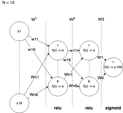
Above picture describes a network we are going to implement.

• N is a number of features, i.e. remaining columns from the input dataset.

• Each layer is fully connected with next layer. I draw each layer by skipping middle neurons to get smaller visual overhead.

• Between each layer we have weights which form linear equations via dot product x * w + bias.

• Each layer has its own activation functions. We use ReLU (Rectified Linear Unit) and Sigmoid functions.

Forward Propagation

Basic idea of neural network implementation is to leverage math principals for matrix and vector multiplication. As neural network is going to be fully connected from layer to layer, we can represent learning and optimization algorithms as following:

Dimensions

Single training example

It is one data record:

1. x: 12 input columns as 1 x 12 matrix
2. w1: 12 x 6 matrix + 6 x 1 matrix for biases
3. w2: 6 x 6 matrix + 6 x 1 matrix for biases
4. w3: 6 x 1 matrix + 1 x 1 matrix for biases
5. yHat: scalar number

An amount of hidden layers and neurons are parameters to be tuned by an expert, i.e. externally to the main algorithm. We set 2 hidden layers with 6 neurons each. Our last layer is single neuron that produces final prediction, which we will treat as yes or no to answer customer churn question.

Multiple training examples

Mini-batch approach, i.e. multiple training examples at once. Batch size to be tuned externally as well. Let's take 16 as batch size:

1. x: 16 x 12 matrix
2. w1: 12 x 6 matrix + 6 x 1 matrix for biases
3. w2: 6 x 6 matrix + 6 x 1 matrix for biases
4. w3: 6 x 1 matrix + 1 x 1 matrix for biases
5. yHat: 16 x 1 matrix

As you can see, our matrices are equal in rows at input and output layers. That means we can input any number of rows through the neural network at once when we do training or prediction.

Math of the Forward propagation

When we train neural network, we use input data and parameters on all hidden layers to reach output layer, so that we get the prediction value(s). First part of the ANN implementation that calculates predictions, i.e. yHat is called _forward propagation.

Linear algebra helps us to feed data into the network and get the result using matrix multiplication principals. That makes the entire training and single prediction quite generic, so that we can easily program that in any programming language.

In a nutshell, our 12 x 6 x 6 x 1 network will form the following expressions for every training batch:

First Hidden Layer

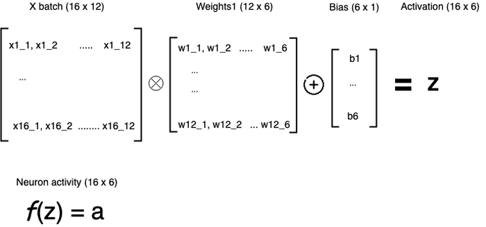
Above picture shows activations for the neurons of the first hidden layer. In fact, next layers are calculated in similar way.

• X is a matrix where each row is a data sample. Every column is a particular feature/column from the initial dataset. Usually, input column is scaled/encoded (see second article).

• We use dot product operation for X and W. Resulting matrix is used to add biases using element-wise addition. b1 will be added to each element of the first row of that resulting matrix, then b2 to the second row and so on.

Second Hidden Layer

The x of the second layer is an a we calculated on the previous layer. We will call it a1.

a1 (16 x 6) * w2 (6 x 6) + b2 (6 x 1) = z2 (16 x 6)

f(z2) = a2 (16 x 6)

Above pseudo-code shows matrix dimensions in the parenthesis.

Output Layer

Input data is a2. Here we get out prediction at the end:

a2 (16 x 6) * w3 (6 x 1) + b3 (1 x 1) = z3 (16 x 1)

f(z3) = a3 (16 x 1)

a3 a.k.a yHat represents a prediction for each data sample in the batch. Prediction values are probabilities between 0 and 1.

If you are confused with above explanation, I recommend to check great video series on Deep Learning: But what is a Neural Network? | Deep learning, chapter 1.

Batch Tracing

In order to see what is going on with the state of neural network, let's feed one single batch into it.

There are different strategies for initial weights and biases initialisation. In our implementation we will follow:

• weight matrices are initialised using uniform-random
• bias vectors are initialised with zeros

Later they will be updated via optimization algorithm.

x - input

Below matrix is our x, which is our input data from the training or test set. The values it contains is a result of data preparation step, which I will explain in details further:

sizes: 16x12, Tensor2D[Float]:
[[-0.032920357,1.1368092,-0.579135,-0.6694619,-0.9335201,0.3765018,-1.0295835,-1.0824665,-0.9476086,0.7312724,0.8284169,-0.05904571]
 [-0.12171035,-0.86240697,-0.579135,1.464448,-0.9335201,0.26486462,-1.3750359,0.2695743,-0.9476086,-1.340666,0.8284169,0.1443363]
 [-0.97732306,1.1368092,-0.579135,-0.6694619,-0.9335201,0.3765018,1.0431306,1.4932814,2.0728939,0.7312724,-1.1834527,0.16957337]
 [0.6128251,1.1368092,-0.579135,-0.6694619,-0.9335201,0.041590314,-1.3750359,-1.0824665,0.5626426,-1.340666,-1.1834527,-0.19572]
 [1.8316696,-0.86240697,-0.579135,1.464448,-0.9335201,0.48813897,-1.0295835,0.94235253,-0.9476086,0.7312724,0.8284169,-0.463582]
 [0.17694691,-0.86240697,-0.579135,1.464448,1.0502101,0.59977615,1.0431306,0.7527129,0.5626426,0.7312724,-1.1834527,0.82049227]
 [1.6056587,1.1368092,-0.579135,-0.6694619,1.0502101,1.2695991,0.69767827,-1.0824665,0.5626426,0.7312724,0.8284169,-1.7176533]
 [-1.9943721,-0.86240697,1.6928561,-0.6694619,-0.9335201,-1.0747813,-0.33867878,0.7735395,3.583145,0.7312724,-1.1834527,0.267966]
 [-0.9853949,1.1368092,-0.579135,-0.6694619,1.0502101,0.59977615,-0.33867878,1.20919,0.5626426,-1.340666,0.8284169,-0.5388685]
 [0.49174783,1.1368092,-0.579135,-0.6694619,1.0502101,-1.2980556,-1.0295835,1.0890474,-0.9476086,0.7312724,0.8284169,-0.5972788]
 [-0.7674558,1.1368092,-0.579135,-0.6694619,1.0502101,-0.85150695,0.35222593,0.563331,0.5626426,-1.340666,-1.1834527,-0.44364995]
 [-1.0176822,-0.86240697,-0.579135,1.464448,1.0502101,-1.6329671,-0.68413115,-1.0824665,0.5626426,0.7312724,-1.1834527,-0.5125319]
 [-1.1871903,1.1368092,-0.579135,-0.6694619,-0.9335201,-0.5165955,1.7340354,-1.0824665,0.5626426,0.7312724,-1.1834527,-1.4233431]
 [-0.5979476,1.1368092,-0.579135,-0.6694619,-0.9335201,-1.52133,0.0067735757,-1.0824665,0.5626426,-1.340666,-1.1834527,1.5672718]
 [0.09622873,-0.86240697,-0.579135,1.464448,-0.9335201,-0.40495834,0.69767827,-1.0824665,0.5626426,0.7312724,0.8284169,-0.70219]
 [-0.05713581,-0.86240697,1.6928561,-0.6694619,1.0502101,0.71141326,-0.68413115,1.2265866,0.5626426,-1.340666,0.8284169,-0.731704]]

w1 - between input and 1st hidden layers

weight:

sizes: 12x6, Tensor2D[Float]:
[[0.0031250487,0.6230519,0.41888618,0.89568454,0.6927525,0.7887961]
 [0.30450296,0.75655645,0.075620584,0.898596,0.66731954,0.06079619]
 [0.21693613,0.89243406,0.6251479,0.080811165,0.30963784,0.87972105]
 [0.006676915,0.05886997,0.88085854,0.29817313,0.19820364,0.6823392]
 [0.73550576,0.49408147,0.99867696,0.71354216,0.9676805,0.09009225]
 [0.19121544,0.021707054,0.53959745,0.74587476,0.16132912,0.08185377]
 [0.2528674,0.562563,0.17039675,0.7291027,0.41844574,0.4336123]
 [0.8275197,0.5867702,0.1692482,0.102723576,0.8936942,0.12275006]
 [0.15337862,0.55374163,0.7993138,0.73106086,0.29611018,0.6279454]
 [0.15933406,0.5840742,0.42520604,0.44090283,0.13000321,0.25581995]
 [0.8168607,0.25407365,0.6668799,0.277898,0.13848923,0.94559854]
 [0.61593276,0.8569094,0.83978665,0.12022303,0.097834654,0.9559516]]

bias:

sizes: 6, Tensor1D[Float]:
[0.0,0.0,0.0,0.0,0.0,0.0]

w2 - between 1st and 2nd hidden layers

weight:

sizes: 6x6, Tensor2D[Float]:
[[0.77492374,0.20006068,0.8301353,0.8226056,0.726444,0.54590976]
 [0.8728169,0.83197665,0.5453676,0.7730933,0.77980715,0.20573096]
 [0.8222075,0.94630164,0.29234344,0.7667057,0.3600455,0.26467463]
 [0.5196553,0.3935514,0.23351222,0.18136671,0.01824836,0.25099826]
 [0.8864608,0.64109814,0.3031471,0.18872173,0.5463185,0.26470202]
 [0.102771536,0.92541504,0.21454614,0.8614344,0.10369446,0.76455885]]

bias:

sizes: 6, Tensor1D[Float]:
[0.0,0.0,0.0,0.0,0.0,0.0]

w3 - between 2nd hidden and output layers

weight:

sizes: 6x1, Tensor2D[Float]:
[[0.63033116]
 [0.6078242]
 [0.022346135]
 [0.62451136]
 [0.89858407]
 [0.5960952]]

bias:

sizes: 1, Tensor1D[Float]:
[0.0]

yHat - Output layer

Predictions for the input batch:

sizes: 16, Tensor1D[Float]:
[0.8810671,0.49800232,0.86774874,0.49800232,0.99999976,0.83703655,0.49800232,0.49800232,0.9976035,0.49800232,0.9999994,0.49800232,0.8031284,0.49800232,0.9775441,0.86094683]

---

Above trace is for the first training batch at the very first epoch. You should not try understand these digits in weights, biases and outputs matrices. They are going to change their values a lot after running training loop 100 times (epochs) with N batches each.

Backward Propagation

Initial weights and biases are not going to give us right equations to predict our y. Even if we propagate the entire dataset through the network. Obviously, someone needs to update these parameters based on some feedback. This feedback is calculated via loss function. In the science literature, loss function is also called as cost function. We are going to use loss and cost here as synonymous.

There are different loss functions in Deep Learning we can use. We will go with binary-cross-entropy as we predict binary value. Our loss value will show how good we are updating the network weights at specific training epoch. However, updates will be done using Gradient Descent optimization algorithm.

Gradient Descent optimization

Model prediction is calculated through the forward propagation of the input data sample(s). If weights and biases are trained well, then our predictions will be accurate as well. In order to say whether our model performs well, we check loss value on every training cycle as well as accuracy metric. Accuracy is number of correct predictions divided by total number of data samples during the training or validation.

You might ask yourself - how can I train model parameters well? In other words how to update them in right direction, so that they give accurate predictions?

Here we meet Gradient Descent.

As per Wikipedia:

Gradient descent is a first-order iterative optimization algorithm for finding a local minimum of a differentiable function

Gradient descent is a way to minimise an objective loss function for neural network parameters. In other words, it helps to find best parameters by minimising loss function. Smaller loss, better overall network accuracy.

Using Gradient Descent, we are finding proper change rate on every training cycle. So that we can update our weights and biases to get the best model performance.

How exactly the Gradient Descent algorithm calculates that change?

There are thousands of articles explaining that visually. In short, we are trying to find steepest descent of the derivative function. Using small coefficient learningRate we subtract the gradient value from the initial parameter. That allows us to find best parameter and minimise the loss function. One of the good visual explanation for linear regression problem with gradient descent is here. It also works well for multiple linear regression like in our case, we got 12 features, so 12 independent variables.

Coming back to our back-propagation implementation. f'(x)is a derivative function of the layer's activation function. We use derivative function to update all weights except the last one, i.e. w1 and w2, not w3. To update w3, we use delta based on the error, i.e. predicted - actual. Layers w1 and w2 are using relu as activation function. Derivative of the relu function is following:

if (x < 0) 0 
else 1

Such derivative function is applied element-wise to z matrix in the step #6 of the back propagation part (see second article for Scala reference implementation).

Math of the Backward propagation

Back-propagation part of ANN is a bit more complicated than forward propagation part. In Gradient Descent Optimization algorithm, we calculate derivatives to calculate yHat rate of change with respect to last z, in our case it is z3.

High-level steps of the Gradient Descent algorithm

0. Calculate error based on actual y and on predicted yHat. It will be called delta further and in the code.

delta = (yHat - y) multiply f'(z)

result is a 16 x 1 matrix

where:
    - "f`" is a derivative to activation function on the current layer.   
    - "z" is current layer activation.
    - "multiply" is Hadamard product, a.k.a. element-wise multiplication. 
      Note: it is not the same as dot product.

1. Iterate list of weights matrices from end to start, i.e. backwards. Let's take "i" as layer index
2. Calculate partial derivative as:

 partialDerivativeN = xi.T * delta

 where:     
     - "T" is a matrix transpose operation,
     - "*" is dot product operation.    

3. Update weights of i layer via:

wi = wi - learningRate * partialDerivative_i 

where:
  - "learningRate" is a scalar number. 
  - "partialDerivative_i" is a matrix, so "*" is dot product here as well.

4. Update bias of i layer via:

bi = bi - sum(delta)

5. Pass updated weight wi and delta to previous layer, i.e. to wi - 1.

6. Now starting wi - 1 weight update, we calculate delta differently.

delta = (previousDelta * previousW) multiply f'(z)

where:
   - "previousDelta" is delta from previous step, i.e. 
      it is from layer next to the right, because we go backward. 
   - "previousW" - is a weight matrix from the previous step as well.

If i > 0, then:

decrement i via i = i -1 and then repeat steps from 2 to 5.

otherwise:

we finished back-propagation for a specific batch or a single data sample (in case of stochastic gradient descent).

Back-propagation tracing

w3 - between 2nd hidden and output layers

Delta (error):

sizes: 16, Tensor1D[Float]:
[-0.5,0.5,-2.336502E-5,0.5,0.99982685,0.0,1.0,-0.27220798,0.9981591,0.99999166,0.5142617,0.5,0.5,0.5,0.5,0.9999994]

x transpose:

sizes: 6x16, Tensor2D[Float]:
[[0.0,0.0,2.3540525,0.0,1.1964836,4.380693,6.6140265,0.44490784,1.8534858,2.7576103,0.007678177,0.0,0.0,0.0,0.0,3.0259452]
 [0.0,0.0,1.4293345,0.0,1.9171724,5.341193,5.351874,0.52522117,1.888961,3.053475,0.0014958136,0.0,0.0,0.0,0.0,4.647504]
 [0.0,0.0,2.901132,0.0,3.4634292,6.8469305,9.681695,0.16261059,1.7458743,4.406227,0.0116603775,0.0,0.0,0.0,0.0,3.5064058]
 [0.0,0.0,2.2631726,0.0,1.4329143,5.5888605,7.362318,0.16618003,1.1314285,2.040889,0.023946803,0.0,0.0,0.0,0.0,2.7598464]
 [0.0,0.0,3.2273922,0.0,2.8001034,8.964131,10.323663,0.10813884,1.4567397,2.918638,0.013493502,0.0,0.0,0.0,0.0,3.6922505]
 [0.0,0.0,3.2367752,0.0,2.513441,9.055562,10.566048,0.26056617,1.7771944,3.133051,0.015981253,0.0,0.0,0.0,0.0,4.64655]]

partialDerivative3 = x.T * (delta multiply f`(z)):

sizes: 6x1, Tensor2D[Float]:
[[15.326693]
 [16.712915]
 [22.761444]
 [14.692074]
 [21.16563]
 [22.569763]]

updated Weight = w - learningRate * partialDerivative3 :

sizes: 6x1, Tensor2D[Float]:
[[0.6776238]
 [0.29685247]
 [0.496793]
 [0.95105153]
 [0.824897]
 [0.64518374]]

updated Bias = b - learningRate * sum(delta) :

sizes: 1, Tensor1D[Float]:
[-0.0077400077]

w2 - between 1st and 2nd hidden layers

current delta:

delta (16x6) = (previous delta * previous w) multiply f`(z)

current derivative:

partialDerivative2 (6 x 6) = x.T (6 x 16) * delta (16 x 6)

updated Weight:

w2 (6x6) = w2 (6x6) - learningRate * partialDerivative2 (6 x 6)

updated Bias:

b2 (6 x 1) = b2 (6 x 1) - learningRate * sum(delta)

w1 - between input and 1st hidden layers

current delta:

delta (16x6) = (previous delta * previous w) multiply f`(z)

current derivative:

partialDerivative1 (12 x 6) = x.T (12 x 16) * delta (16 x 6)

updated Weight:

w1 (12x6) = w2 (12x6) - learningRate * partialDerivative1 (12 x 6)

updated Bias:

b1 (6 x 1) = b1 (6 x 1) - learningRate * sum(delta)

Wrapping up

We have finished with theoretical part and ready to continue with the second article ANN in Scala: implementation. In case you have not gotten how the ANN is actually working in theory, then I encourage you to search for other articles and videos. It is important to understand this part before looking at actual implementation in code.