MNIST image recognition using Deep Feed Forward Network
Deep Feed Forward Neural Network is one of the type of Artificial Neural Networks, which is also able to classify computer images. In order to feed pixel data into the neural net in RBG/Greyscale/other format one can map every pixel to network inputs. That means every pixel becomes a feature. It may sound scary and highly inefficient to feed, let's say, 28 hieght on 28 width image size, which is 784 features to learn from. However, neural networks can learn from the pixel data successfully and classify unseen data. We are going to prove this.
Please note, there are additional type of networks which are more efficient in image classification such as Convolutional Neural Network, but we are going to talk about that next time.
Dataset

MNIST dataset is a "Hello, World!" dataset in the field of Deep Learning. It consists of thousands of grey-scaled images which represent hand-written digits from 0 to 9, so 10 labels. This dataset is used by many researches in the field to evaluate their discoveries and test that on well-known dataset. However, MNIST dataset should not be a panacea. There are other public datasets with images like ImageNet, AlexNet, etc., which are more advanced as they have more objects than just hand-written digits. Nevertheless, MNIST made important contribution to the history of Deep Learning and still helps people to learn this field by playing with this dataset.
Loading Data
MNIST dataset can be taken from Yann LeCun web-site: http://yann.lecun.com/exdb/mnist/. If it is unavailable, you can easily find
a copy of this dataset in numerous GitHub repositories, since it is not big in size (for example here). I have downloaded the following 4 archives and put into the folder images.
9.5M train-images-idx3-ubyte.gz
28K  train-labels-idx1-ubyte.gz

1.6M t10k-images-idx3-ubyte.gz
4.4K t10k-labels-idx1-ubyte.gz
First two files is training dataset. Bigger file is for images and smaller is for labels. There are 60000 training images and labels for them. Next two files are for model testing following the same concept (images, labels). There are 10000 testing images and labels.
In order to load these files into the memory we need to follow MNIST file format specification. For each file we need to do:
- Read first magic number and compare it with MNIST expected number, which is:
val LabelFileMagicNumber = 2049
val ImageFileMagicNumber = 2051- Read next number for number of rows
- Read next number for number of columns
- Read images and labels in the loop based on the number of rows and columns
We are going to implement MNIST classification on top of the existing mini-libary for Deep Learning. Here is how we can load MNIST dataset:
import scala.collection.mutable.ArrayBuffer
import scala.reflect.ClassTag

import java.io.{DataInputStream, BufferedInputStream, FileInputStream}
import java.nio.file.{Files, Path}
import java.util.zip.GZIPInputStream

def loadDataset[T: ClassTag](images: Path, labels: Path)(
    using n: Numeric[T]
  ): (Tensor[T], Tensor[T]) =

  val imageStream = new GZIPInputStream(Files.newInputStream(images))
  val imageInputStream = new DataInputStream(new BufferedInputStream(imageStream))
  val magicNumber = imageInputStream.readInt()

  assert(magicNumber == ImageFileMagicNumber,
    s"Images magic number is incorrect, expected $ImageFileMagicNumber,
    but was $magicNumber")

  val numberOfImages = imageInputStream.readInt()
  val (nRows, nCols) = (imageInputStream.readInt(), imageInputStream.readInt())

  val labelStream = new GZIPInputStream(Files.newInputStream(labels))
  val labelInputStream = new DataInputStream(new BufferedInputStream(labelStream))
  val labelMagicNumber = labelInputStream.readInt()

  assert(labelMagicNumber == LabelFileMagicNumber,
    s"Labels magic number is incorrect, expected $LabelFileMagicNumber,
    but was $labelMagicNumber")

  val numberOfLabels = labelInputStream.readInt()

  assert(numberOfImages == numberOfLabels)

  val labelsTensor = labelInputStream.readAllBytes.map(l => n.fromInt(l)).as1D

  val singeImageSize = nRows * nCols
  val imageArray = ArrayBuffer.empty[Array[T]]

  for i <- (0 until numberOfImages) do
    val image = (0 until singeImageSize)
      .map(_ => n.fromInt(imageInputStream.readUnsignedByte())).toArray
    imageArray += image

  (imageArray.toArray.as2D, labelsTensor)
Preparing data
Before we construct a neural network to train it on MNIST dataset, we need to transform it a bit.
Feature normalisation
In order to be more efficient when learning weights we need to scale X data to be in [0, 1] data range. We know that every image is encoded as a matrix of pixels 28 x 28. If print one of the image data into the console with line breaks after 28-th element, then it will look like this:
0   0   0   0   0   0   0   0   0   0   0   0   0   0   0   0   0   0   0   0   0   0   0   0   0   0   0   0
0   0   0   0   0   0   0   0   0   0   0   0   0   0   0   0   0   0   0   0   0   0   0   0   0   0   0   0
0   0   0   0   0   0   0   0   0   0   0   0   0   0   0   0   0   0   0   0   0   0   0   0   0   0   0   0
0   0   0   0   0   0   0   0   0   0   0   0   0   0   0   0   0   0   0   0   0   0   0   0   0   0   0   0
0   0   0   0   0   0   0   0   0   0   0   0   0   0   0   0   0   0   0   0   0   0   0   0   0   0   0   0
0   0   0   0   0   0   0   0   0   0   0   0   0   0   0   0   0   0   0   0   0   0   0   0   0   0   0   0
0   0   0   0   0   0   0   0   0   0   0   0   0   0   0   0   0   0   0   0   0   0   0   0   0   0   0   0
0   0   0   0   0   0  84 185 159 151  60  36   0   0   0   0   0   0   0   0   0   0   0   0   0   0   0   0
0   0   0   0   0   0 222 254 254 254 254 241 198 198 198 198 198 198 198 198 170  52   0   0   0   0   0   0
0   0   0   0   0   0  67 114  72 114 163 227 254 225 254 254 254 250 229 254 254 140   0   0   0   0   0   0
0   0   0   0   0   0   0   0   0   0   0  17  66  14  67  67  67  59  21 236 254 106   0   0   0   0   0   0
0   0   0   0   0   0   0   0   0   0   0   0   0   0   0   0   0   0  83 253 209  18   0   0   0   0   0   0
0   0   0   0   0   0   0   0   0   0   0   0   0   0   0   0   0  22 233 255  83   0   0   0   0   0   0   0
0   0   0   0   0   0   0   0   0   0   0   0   0   0   0   0   0 129 254 238  44   0   0   0   0   0   0   0
0   0   0   0   0   0   0   0   0   0   0   0   0   0   0   0  59 249 254  62   0   0   0   0   0   0   0   0
0   0   0   0   0   0   0   0   0   0   0   0   0   0   0   0 133 254 187   5   0   0   0   0   0   0   0   0
0   0   0   0   0   0   0   0   0   0   0   0   0   0   0   9 205 248  58   0   0   0   0   0   0   0   0   0
0   0   0   0   0   0   0   0   0   0   0   0   0   0   0 126 254 182   0   0   0   0   0   0   0   0   0   0
0   0   0   0   0   0   0   0   0   0   0   0   0   0  75 251 240  57   0   0   0   0   0   0   0   0   0   0
0   0   0   0   0   0   0   0   0   0   0   0   0  19 221 254 166   0   0   0   0   0   0   0   0   0   0   0
0   0   0   0   0   0   0   0   0   0   0   0   3 203 254 219  35   0   0   0   0   0   0   0   0   0   0   0
0   0   0   0   0   0   0   0   0   0   0   0  38 254 254  77   0   0   0   0   0   0   0   0   0   0   0   0
0   0   0   0   0   0   0   0   0   0   0  31 224 254 115   1   0   0   0   0   0   0   0   0   0   0   0   0
0   0   0   0   0   0   0   0   0   0   0 133 254 254  52   0   0   0   0   0   0   0   0   0   0   0   0   0
0   0   0   0   0   0   0   0   0   0  61 242 254 254  52   0   0   0   0   0   0   0   0   0   0   0   0   0
0   0   0   0   0   0   0   0   0   0 121 254 254 219  40   0   0   0   0   0   0   0   0   0   0   0   0   0
0   0   0   0   0   0   0   0   0   0 121 254 207  18   0   0   0   0   0   0   0   0   0   0   0   0   0   0
0   0   0   0   0   0   0   0   0   0   0   0   0   0   0   0   0   0   0   0   0   0   0   0   0   0   0   0
Above output corresponds to digit "7".
Data in 0-255 numeric range will explode our network gradient if we do not apply any optimization technique on gradient or weight values. The easiest way is to scale the input data.
First we load data using previously defined function with one more case class as a wrapper:
val dataset = MnistLoader.loadData[Double]("images")where dataset is wrapped into a case class:
case class MnistDataset[T: Numeric](
  trainImage: Tensor[T],
  trainLabels: Tensor[T],
  testImages: Tensor[T],
  testLabels: Tensor[T])
Then we simply divide every value by 255, that gives data in [0,1] range format.
val xData = dataset.trainImage.map(_ / 255d) Target Encoding
Our model is going to predict one label over multi-class dataset. In order to make our neural network
to predict something we need to encode label tensor with One-Hot encoder, so that every scalar label becomes as
a vector of zeros and a single 1. Index of 1 corresponds to the digit that this label stores.
MNIST data is currently a vector of numbers, where number is a label for hand-written digit. For example:
[7,5,0,1]Once we one-hot encode it, it will look like:
[0,0,0,0,0,0,0,1,0,0]
[0,0,0,0,0,1,0,0,0,0]
[1,0,0,0,0,0,0,0,0,0]
[0,1,0,0,0,0,0,0,0,0]
We can reuse OneHotEncoder implemented earlier:
val encoder = OneHotEncoder(classes = (0 to 9).map(i => (i.toDouble, i.toDouble)).toMap)
val yData = encoder.transform(dataset.trainLabels.as1D)
Common preparation
Let's wrap both transformation into one function:
def prepareData(x: Tensor[Double], y: Tensor[Double]) =
  val xData = x.map(_ / 255d) // normalize to [0,1] range
  val yData = encoder.transform(y.as1D)
  (xData, yData)
Now we can call it like this:
val (xTrain, yTrain) = prepareData(dataset.trainImage, dataset.trainLabels)Model construction
Our model is going to be designed/trained with:
- nodes: 784 x 100 x 10
- activation: ReLU, Softmax
- loss: cross-entropy
- accuracy: via argmax
- initialisation: Kaiming
- optimizer: Adam
val ann = Sequential[Double, Adam, HeNormal](
  crossEntropy,
  learningRate = 0.001,
  metrics = List(accuracy),
  batchSize = 128,
  gradientClipping = clipByValue(5.0d)
)
  .add(Dense(relu, 100))
  .add(Dense(softmax, 10))
Adam optimizer gets better results on MNIST data, so we stick to it, rather than with standard Stochastic Gradient Descent.
Activations
We have already seen ReLU activation function, but let's recall its definition:
def relu[T: ClassTag](x: Tensor[T])(using n: Numeric[T]): Tensor[T] =
  x.map(t => max(n.zero, t))
Important note here that it is applied element-wise, i.e. for every element of z matrix in the layer.
However, softmax activation function is applied across nodes of the layer to get the probability which sums up to 1.
This activation function is a typical choice for multi-class problem type. When we feed input data sample into the network,
we want to get an output as vector with probabilities for each class.
Coming back to MNIST target, below representation shows that most likely the target value is digit "4", because the highest argument is "0.5" at index [4].
scala> List(0.01, 0.2, 0.1, 0.1, 0.5, 0.01, 0.02, 0.03, 0.01, 0.02).sum
val res0: Double = 1.0
This is how we can implement softmax:
val toleration = castFromTo[Double, T](0.4E-15d)

def softmax(x: Tensor[T]): Tensor[T] =
  val applied = x.mapRow { row =>
    val max = row.max
    val expNorm = row.map(v => exp(v - max))
    val sum = expNorm.sum
    expNorm.map(_ / sum)
  }

  // rest is an extra defence against numeric overflow
  val appliedSum = applied.sumCols.map( v =>
    if v.abs - toleration > n.one
    then v
    else n.one
  )
  val totalSum = appliedSum.sumRows.as0D.data
  assert(totalSum == x.length,
    s"Softmax distribution sum is not equal to 1 at some activation, but\n${appliedSum}")

  applied
It is obviously more complicated than relu. This is what the above code is doing:
- For each
row: Array[T]of thexTensor we find a max value and substract it from each value of this row to get stable values in the vector. The reason to subtractmaxis to avoid numeric overflow. - Apply exponent to each value right after the
maxsubtraction. - Make a sum of exponents.
- Finally, use exponent vector to divide each value by the
sum. - Additionally, we raise an error if a sum of individual values in
the vector is not equal to
1. Such situation may happen due to numeric overflow. If it happens, then we may end up with exploding gradient (as a result bad training outcome). However, we tolerate numeric difference of0.4E-15d, i.e. it should be no more than1.0000000000000004.
In order to perform back-propagation with gradient descent we need softmax derivative as well.
This is simplest version of softmax derivative:
def derivative(x: Tensor[T]): Tensor[T] =
  val sm = softmax(x)
  sm.multiply(n.one - sm) // element-wise multiplication, NOT dot product
Loss function
Cross-entropy can then be used to calculate the difference between the two probability distributions and
typical choice for multi-class classification. It can written in code as:
def crossEntropy[T: ClassTag: Numeric](y: T, yHat: T): T =
  y * log(yHat)
It will return some value as a as difference. Example of input vectors:
some random yHat = [0.1, 0.1, 0, 0.8, ...] - it will be length of 10 in our MNIST case
        actual y = [0, 0, 0, 1, ........ ] - length 10
To get an idea whey cross-entropy is a usefull loss function to our problem, please have a look at this blog-post.
Accuracy
Before we calculate a number of correct predictions, we need to not just compare y and yHat vectors,
but first need to find an index of the max element in the y and yHat vectors.
So we need to help the existing algorithm to extract from the yHat vector the value of the label, i.e. predicted digit.
Function called argmax can be used for this task:
def accuracyMnist[T: ClassTag: Ordering](using n: Numeric[T]) = new Metric[T]:
  val name = "accuracy"

  def matches(actual: Tensor[T], predicted: Tensor[T]): Int =
    val predictedArgMax = predicted.argMax
    actual.argMax.equalRows(predictedArgMax)

val accuracy = accuracyMnist[Double]
Accuracy is a Metric type-class that has matches method to return a number of correct predictions.
The argMax itself as generic tensor function:
def argMax[T: ClassTag](t: Tensor[T])(using n: Numeric[T]) =
  def maxIndex(a: Array[T]) =
    n.fromInt(a.indices.maxBy(a))

  t match
    case Tensor2D(data) => Tensor1D(data.map(maxIndex))
    case Tensor1D(data) => Tensor0D(maxIndex(data))
    case Tensor0D(_) => t
Weight Initialisation
Weight initialisation approach is important factor in Deep Learning to converge model training faster or even to avoid vanished or exploded gradient.
Kaiming weight initialisation is helping to address above problems. So let's use that as well:
given [T: ClassTag: Numeric]: ParamsInitializer[T, HeNormal] with
  val rnd = new Random()

  def gen(lenght: Int): T =
    castFromTo[Double, T]{
      val v = rnd.nextGaussian + 0.001d // value shift is optional
      v * math.sqrt(2d / lenght.toDouble)
    }

  override def weights(rows: Int, cols: Int): Tensor[T] =
    Tensor2D(Array.fill(rows)(Array.fill[T](cols)(gen(rows))))

  override def biases(length: Int): Tensor[T] =
    zeros(length)
We initialise biases to zeros. Weight matrices are initialised using random generator with normal distribution. Every random number then
multiplied by sqrt(2 / n), where n is a number of input nodes for this particular layer.
Model Training
Now we are ready to start training process.
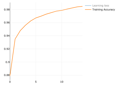
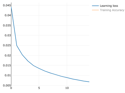
val model = ann.train(xTrain, yTrain, epochs = 15, shuffle = true) epoch: 1/15, avg. loss: 0.04434336993179046, metrics: [accuracy: 0.8785666666666667]
epoch: 2/15, avg. loss: 0.024939809896450383, metrics: [accuracy: 0.9350166666666667]
epoch: 3/15, avg. loss: 0.02028075875579972, metrics: [accuracy: 0.9478833333333333]
epoch: 4/15, avg. loss: 0.017196840063260558, metrics: [accuracy: 0.9560833333333333]
epoch: 5/15, avg. loss: 0.01491209973340988, metrics: [accuracy: 0.9625666666666667]
epoch: 6/15, avg. loss: 0.01350024657628137, metrics: [accuracy: 0.9671833333333333]
epoch: 7/15, avg. loss: 0.01222168129663168, metrics: [accuracy: 0.9699]
epoch: 8/15, avg. loss: 0.011222418180870991, metrics: [accuracy: 0.9729833333333333]
epoch: 9/15, avg. loss: 0.010388172803460627, metrics: [accuracy: 0.9752833333333333]
epoch: 10/15, avg. loss: 0.009549474708521941, metrics: [accuracy: 0.97765]
epoch: 11/15, avg. loss: 0.008920235294999721, metrics: [accuracy: 0.9787]
epoch: 12/15, avg. loss: 0.008214811390229967, metrics: [accuracy: 0.9806833333333334]
epoch: 13/15, avg. loss: 0.0077112882811408694, metrics: [accuracy: 0.9824]
epoch: 14/15, avg. loss: 0.0071559669134910325, metrics: [accuracy: 0.98405]
epoch: 15/15, avg. loss: 0.006797865863855411, metrics: [accuracy: 0.9848]We have gotten quite good accuracy on training. 98.4% correct predictions, which is 1.6% errors.
Model Testing
val (xTest, yTest) = prepareData(dataset.testImages, dataset.testLabels)
val testPredicted = model(xTest)
val value = accuracy(yTest, testPredicted)
println(s"test accuracy = $value")
Accuracy on test data is quite close to the train accuracy:
test accuracy = 0.9721We can also try to run a single test on the first image from the test dataset:
val singleTestImage = dataset.testImages.as2D.data.head
val label = dataset.testLabels.as1D.data.head // this must be "7"
val predicted = model(singleTestImage.as2D).argMax.as0D.data

assert(label == predicted,
  s"Predicted label is not equal to expected '$label' label, but was '$predicted'")

println(s"predicted = $predicted")
predicted = 7.0Summary
We have seen that even one hidden layer is able to classify MNIST dataset with quite low error rate. Key takeaways when classifying images are:
- make sure that gradient is not going to explode or vanish. For that, we can use proper weight initialisation, clipping gradient by value or norm any other weight normalisation during the training. Also scale or normalise the input data
- use one-hot encoding for your target variable in case of multi-class classification
- in case of single label prediction, use
argmaxfunction - use
softmaxactivation at the last layer to distribute probabilities across classes.
Try Convolutional Neural Network as a next step in image classification problem.