Last time we used ANN to train a Deep Learning model for image recognition using MNIST dataset. This time we are going to look at more advanced network called Convolutional Neural Network or CNN in short.

CNN is designed to tackle image recognition problem. However, it can be used not only for image recognition. As we have seen last time, ANN using just hidden layers can learn quite well on MNIST. However, for real life use cases we need higher accuracy. The main idea of CNN is to learn how to recognise object in their different shapes and positions using specific features of the image data. The goal of CNN is better model regularisation by using convolution and pooling operations.

CNN adds two more type of layers:

• Convolution layer
• Max, Average or Global Pooling layer

Convolution is a mathematical operation, which is used in CNN layers instead of matrix multiplication like in fully-connected (dense) layers. Typical CNN may consist of several Convolutional and Pooling layers. Final part of the network consists of the fully-connected layers like in ANN.

Below picture is showing typical CNN architecture with Tensor shapes. For example, 32x32x1 is an input image 32 pixels width and height having 1 color channel:

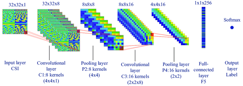
I will clarify what other shapes dimensions mean further.

CNN Topology

We are going to design a simple CNN architecture for image recognition of the MNIST dataset. The problem type will be still the same: predict a hand-written digit based on input image data. CNN works with image properties like height, width and color depth (RGB, etc.). Basically, it uses image pixel matrices to perform convolution and pooling operations. CNN works with every color channel separately. After some point, channels add up to each other using element-wise addition.

I am going to build CNN using my existing mini-library in Scala:

val cnn = Sequential[Precision, Adam, HeNormal](
    crossEntropy,
    learningRate = 0.001,
    metrics = List(accuracy),
    batchSize = 128,
    gradientClipping = clipByNorm(5.0),
    printStepTps = true
  )    
    .add(Conv2D(relu, 8, kernel = (5, 5), strides = (1, 1)))    
    .add(MaxPool(strides = (1, 1), pool = (2, 2), padding = false))       
    .add(Flatten2D())
    .add(Dense(relu, 50))      
    .add(Dense(softmax, 10))

There are 3 more layers that we have not seen before.

Convolution Layer

Conv2D is a Scala case class which has already familiar to us relu parameter as an activation function. Other unique parameters of convolution layer:

• filterCount = 8 - number of filters which are going to be trained/optimised via gradient descent and back-propagation
• kernel = (5, 5) - window height and width to apply on input image/matrix
• strides = (1, 1) - increment value when moving filter over the input image/matrix to the right (1 and to the bottom 1)

While implementing CNN we are going to enter the world of 4-dimensional tensors. Conv2D layer will keep its data in 4D Tensor where:

• 1st dimension is filter count
• 2nd - color depth. Grey scale image is 1, RGB is 3, RGBA is 4 and so on.
• 3rd - filter height
• 4th - filter width

According to above code snippet, added filter will have the following trainable weights and biases:

• weights shape: (8 x 1 x 5 x 5) Tensor4D
• biases shape: (8) Tensor1D

Example

If we take simple example as image matrix 3 x 4 and filter with weights set from 1 to 4 then we get the following output as z:

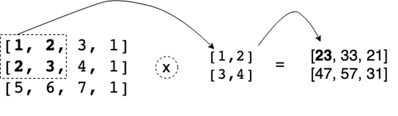
z value at (0, 0) position is elementwise multiplication and then sum of the elements of the matrix such as
1 * 1 + 2 * 2 + 3 * 2 + 3 * 4 = 23. Other output elements of the z matrix are produced in the same way.

Every layer that we add to Sequential model has at least two methods apply, which is used to do forward propagation and backward for producing gradients based on the layer input data.

We can code forward propagation like this:

// create input image regions with their positions to be used by other functions
private def imageRegions(image: Tensor2D[T], kernel: (Int, Int), stride: (Int, Int)) =
  val (rows, cols) = image.shape2D    
  for i <- 0 to rows - kernel._1 by stride._1 yield   
  for j <- 0 to cols - kernel._2 by stride._2 yield       
    (image.slice((i, i + kernel._1), (j, j + kernel._2)).as2D, i, j)

// convolution operation which is
// element-wise multiplication between each image region and filter matrix
private def conv(filterChannel: Tensor2D[T], imageChannel: Tensor2D[T], 
         kernel: (Int, Int), stride: (Int, Int)) =    
  val filtered = 
    for row <- imageRegions(imageChannel, kernel, stride) yield
      for (region, _, _) <- row yield
        (region |*| filterChannel).sum

  filtered.as2D

// main forward function which is used by Conv2D layer to 
// apply every filter channel matrix to every input image.
// N.B. convoluted channels adds us together
private def forward(kernel: (Int, Int), stride: (Int, Int), 
  x: Tensor[T], w: Tensor[T], b: Tensor[T]): Tensor[T] =
  val (images, filters) = (x.as4D, w.as4D)    
   
  def filterImage(image: Array[Array[Array[T]]]) =
    filters.data.zip(b.as1D.data).map { (f, b) =>
      val filtered = f.zip(image).map { (fc, ic) =>
         conv(fc.as2D, ic.as2D, kernel, stride)
      }.reduce(_ + _)
      filtered + b.asT
    }
   
  images.data.par.map(filterImage).toArray.as4D

 // Layer interface to the training loop. 
 // `w` and `b` are the Layer state.
 override def apply(x: Tensor[T]): Activation[T] =
   val z = (w, b) match
     case (Some(w), Some(b)) => forward(kernel, strides, x, w, b)
     case _ => x // does nothing when one of the params is empty    
   val a = f(z)    
   Activation(x, z, a)

I have left private modifier to show you that apply function uses other functions internally.

In general, forward propagation of the Convolution layer is not that simple as for Dense layer. Convolution layer is also computationally intensive in forward and backward propagation.

The main line of code in forward propagation is (region |*| filterChannel).sum. It corresponds to element-wise multiplication of two matrices and summing the resulting matrix up to get single number as one of the value for the output matrix.

Tensor shape of the forward propagation can be calculated in advance using the following formula:

val rows = (height - kernel._1) / strides._1 + 1
val cols = (width - kernel._2) / strides._2 + 1
// final output shape after layer activation is
val shape = List(images, filterCount, rows, cols)

images is a number of images passed via apply, i.e. during the forward propagation. That means we can process a batch of images at once, i.e. at a step. We use similar idea in Dense layers via 2D Tensor to pass multiple images as rows at once (see further).

Pooling Layer

Typical pooling layer that is used for CNN is Max Pooling. As denoted by its name, it pools maximum elements from some image region to place it into the output matrix.

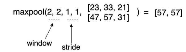
Although above example is quite simple, it shows the idea how forward propagation of MaxPool layer works. Basically, it downsamples input image resolution and takes the most bright pixels.

Here is how we can code max pooling forward propagation:

// shape2D is output shape of this layer
// this function creates image regions from the input X
private def imageRegions(image: Tensor2D[T], window: (Int, Int), strides: (Int, Int)) =
  val (rows, cols) = shape2D
  for i <- 0 until rows by strides._1 yield   
    for j <- 0 until cols by strides._2 yield          
      (image.slice((i, i + window._1), (j, j + window._2)).as2D, i, j)

// main function to find max element in the region
private def poolMax(image: Tensor2D[T]): Tensor2D[T] =
  val (rows, cols) = shape2D
  val out = Array.ofDim(rows, cols)
  val pooled = 
    for (region, i, j) <- imageRegions(image, window, strides).flatten yield            
      out(i)(j) = region.max
  out.as2D

// Layer interface to forward propagation
def apply(x: Tensor[T]): Activation[T] =    
  val pooled = x.as4D.data.map(_.map(c => poolMax(c.as2D))).as4D
  Activation(x, pooled, pooled)

Flatten2D

Before we feed intermediate data from the Convolution and Pooling layers forward, we need to flatten every image to a vector. Image channels are going to be appended to each other to get a single vector per image. Our Tensor4D becomes a Tensor2D, where every row is an image. It is going to be still a long row per image, but since we have done some convolutions on the input image, such processed data helps a model to learn better and avoid overfitting. Again, real-life CNN network will have multiple convolution and pooling layers, which are not necessarily decrease amount of features, but transform them to achieve better model regularisation.

This layer forward propagation is going to be very simple to implement:

def apply(x: Tensor[T]): Activation[T] =
  val flat = x.as2D
  Activation(x, flat, flat)

Where .as2D is combining all nested arrays of 4D Tensor starting from axis = 1.

When we flatten input data we get 4232 long vector image. To summarise the Tensor shapes we get the following output shapes:

• Conv2D shape: 128 x 8 x 24 x 24
• MaxPool shape: 128 x 8 x 23 x 23
• Flatten: 128 x 4232
• Dense shape: 128 x 32
• Dense shape: 128 x 1

Summary

If I run training for 5 epochs it takes a lot time than before with ANN.

val model = cnn.train(xTrain, yTrain, epochs = 5, shuffle = true)

First of all we have more feature now with CNN = 4232 to learn in fully-connected layers. But the main slowness comes from the forward and backward computation of the convolutional and pooling layers. They are much slower than simple dense layer matrix multiplication.

This takes up to 1 hour to train on MNIST on 50k images. The highest accuracy score I got was 92%, which is much lower than with ANN = 98.5%. As we have too few layers and most probably exploding/vanishing gradient I could not better result with CNN. However, it is quite possible to get that with production libraries like Tensorflow, where you will get 98% accuracy or higher using the same architecture that I used in this article.

If you are curious to know how back-propagation is done for Flatten, MaxPool and Conv layers feel free to look at the code of backward methods here.

Links

1. Library source code
2. CNN Figure